37 RELATIVITY
37.1 Invariance of Physical laws
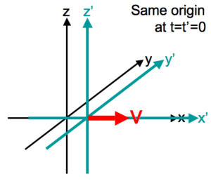
Einstein’s First Postulate (principle of relativity): The laws of physics are the same in every inertial frame of reference.
Einstein’s Second Postulate: The speed of light in vacuum is the same in all inertial frames of reference and is independent of the motion of the source.
37.2 Relativity of Simultaneity

37.3 Relativity of Time Interval
 \[
Time\ dilation:\underbrace{\Delta t}_{Time\ interval\ between\ same\ events\\ measured\ in\ second\ frame\ of\ reference}=\frac{\overbrace{\Delta t_{0}}^{Proper\ time\ between\ two\ events\ (measured\ in\ rest\ frame)}}{\sqrt{1-u^{2} / c^{2}}}
\]
\[
Time\ dilation:\underbrace{\Delta t}_{Time\ interval\ between\ same\ events\\ measured\ in\ second\ frame\ of\ reference}=\frac{\overbrace{\Delta t_{0}}^{Proper\ time\ between\ two\ events\ (measured\ in\ rest\ frame)}}{\sqrt{1-u^{2} / c^{2}}}
\]
37.4 Relativity of Length

37.5 The Lorentz Transformations

37.6 The Doppler Effect For Electromagnetic Waves

37.7 Relativistic Momentum
Relativistic momentum \[ \vec{p}=\frac{m \vec{v}}{\sqrt{1-v^{2} / c^{2}}} \]
37.8 Relativistic Work And Energy
Relativistic kinetic energy \[ K=\frac{m c^{2}}{\sqrt{1-v^{2} / c^{2}}}-m c^{2}=(\gamma-1) m c^{2} \] Total energyof a particle \[ E=K+m c^{2}=\frac{m c^{2}}{\sqrt{1-v^{2} / c^{2}}}=\gamma m c^{2} \] Total energy, rest energy, and momentum \[ \overbrace{E^{2}}^{Total\ energy}=\overbrace{\left(m c^{2}\right)^{2}}^{Rest\ energy}+\overbrace{\left(p_{2}\right)^{2}}^{Magnitude\ of\\momentum} \]
37.9 Newtonian Mechanics And Relativity
Correspondence principle

One test has to do with understanding the rotation of the axes of the planet Mercury’s elliptical orbit, called the precession of the perihelion. (The perihelion is the point of closest approach to the sun.)

Each planet orbiting the Sun follows an elliptic orbitthat gradually rotates over time (apsidal precession). This figure illustrates positive apsidal precession (advance of the perihelion), with the orbital axis turning in the same direction as the planet's orbital motion. The eccentricity of this ellipse and the precession rate of the orbit are exaggerated for visualization. Most orbits in the Solar System have a much lower eccentricity and precess at a much slower rate, making them nearly circular and stationary. A second test concerns the apparent bending of light rays from distant stars when they pass near the sun.

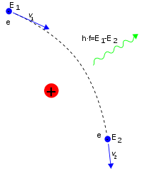
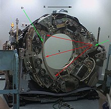
One of Eddington's photographs of the 1919 solar eclipse experiment, presented in his 1920 paper announcing its success The third test is the gravitational red shift, the increase in wavelength of light pro-ceeding outward from a massive source.

The gravitational redshift of a light wave as it moves upwards against a gravitational field (caused by the yellow star below).
38 PHOTONS: LIGHT WAVES BEHAVING AS PARTICLES

- Low-energy phenomena: Photoelectric effect
- Mid-energy phenomena: Thomson scattering/Compton scattering
- High-energy phenomena: Pair production
38.1 Light Absorbed As Photons: The Photoelectric Effect

38.2 Light Emitted As Photons: X-Ray Production
38.3 Light Scattered As Photons: Compton Scattering And Pair Production


38.4 Wave–Particle Duality, Probability, And Uncertainty
Uncertainty principle
- Heisenberguncertainty principle forposition and momentum:
\[ \Delta x \Delta p_{x} \geq \hbar / 2 \]
- Heisenberguncertainty principle forenergy and time:
\[ \Delta t \Delta E \geq \hbar / 2 \]
39 PARTICLES BEHAVING AS WAVES
39.1 Electron Waves
Electron diffraction
Electron microscope
39.2 The Nuclear Atom And Atomic Spectra

39.3 Energy Levels And The Bohr Model Of The Atom

39.4 The Laser


39.5 Continuous Spectra


Planck radiation law \[ I(\lambda)=\frac{2 \pi h c^{2}}{\lambda^{5}\left(e^{h c / \lambda k T}-1\right)} \]
39.6 The Uncertainty Principle Revisited
40 QUANTUM MECHANICS I: WAVE FUNCTIONS
40.1 Wave Functions And The One-Dimensional Schrödinger Equation


General one-dimensional Schrödinger equation: \[
-\frac{\hbar^{2}}{2 m} \frac{\partial^{2} \Psi(x, t)}{\partial x^{2}}+U(x) \Psi(x, t)=i \hbar \frac{\partial \Psi(x, t)}{\partial t}
\] Time-independent one-dimensional Schrödinger equation: \[
-\frac{\hbar^{2}}{2 m} \frac{d^{2} \psi(x)}{d x^{2}}+U(x) \psi(x)=E \psi(x)
\] 
40.2 Particle in a Box

40.3 Potential Wells
Finite potential well
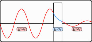
40.4 Potential Barriers and tunneling
applications of tunneling: tunnel diode & Josephson junction in quantum computing
Quantum dot Quantum wire
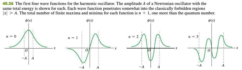
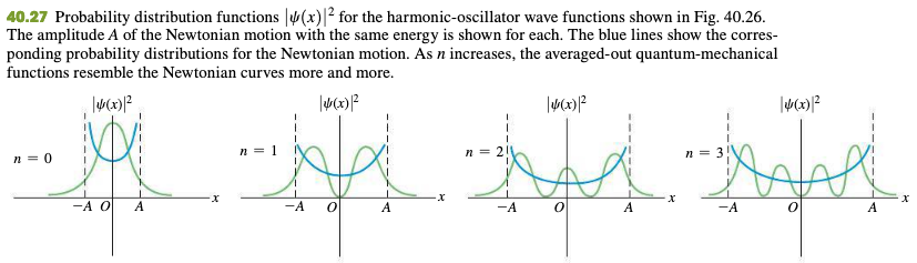
40.5 The Harmonic Oscillator
Hermite function
40.6 Measurement In Quantum Mechanics
Measuring a physical property of a system can change the wave function of that system.
wave-function collapse
many-worlds interpretation

The quantum-mechanical "Schrödinger's cat" theorem according to the many-worlds interpretation. In this interpretation, every event is a branch point; the cat is both alive and dead, even before the box is opened, but the "alive" and "dead" cats are in different branches of the universe, both of which are equally real, but which do not interact with each other.
41 QUANTUM MECHANICS II: ATOMIC STRUCTURE
41.1 The Schrödinger Equation In Three Dimensions
Time-independent three-dimensional Schrödinger equation: \[ \begin{aligned}-\frac{\hbar^{2}}{2 m}\left(\frac{\partial^{2} \psi(x, y, z)}{\partial x^{2}}\right.&+\frac{\partial^{2} \psi(x, y, z)}{\partial y^{2}}+\frac{\partial^{2} \psi(x, y, z)}{\partial z^{2}} ) +U(x, y, z) \psi(x, y, z)=E \psi(x, y, z) \end{aligned} \]
41.2 Particle In A Three-Dimensional Box
\[ E_{n_{X}, n_{Y}, n_{Z}}=\frac{\left(n_{X}^{2}+n_{Y}^{2}+n_{Z}^{2}\right) \pi^{2} \hbar^{2}}{2 m L^{2}} \]
41.3 The Hydrogen Atom
The Schrödinger equation for the hydrogen atom: \[
\begin{aligned}-\frac{\hbar^{2}}{2 m_{\mathrm{r}} r^{2}} \frac{d}{d r}\left(r^{2} \frac{d R(r)}{d r}\right)+\left(\frac{\hbar^{2} l(l+1)}{2 m_{\mathrm{r}} r^{2}}+U(r)\right) R(r) &=E R(r) \\ \frac{1}{\sin \theta} \frac{d}{d \theta}\left(\sin \theta \frac{d \Theta(\theta)}{d \theta}\right)+\left(l(l+1)-\frac{m_{l}^{2}}{\sin ^{2} \theta}\right) \Theta(\theta) &=0 \\ \frac{d^{2} \Phi(\phi)}{d \phi^{2}}+m_{l}^{2} \Phi(\phi) &=0 \end{aligned}
\] Energy levels of hydrogen:principal quantum number \[
E_{n}=-\frac{1}{\left(4 \pi \epsilon_{0}\right)^{2}} \frac{m_{\mathrm{r}} e^{4}}{2 n^{2} \hbar^{2}}=-\frac{13.60 \mathrm{eV}}{n^{2}}
\] Magnitude of orbital angular momentum, hydrogen atom:orbital quantum number \[
L=\sqrt{l(l+1) \hbar} \quad(l=0,1,2, \ldots, n-1)
\] z-component of orbital angular momentum, hydrogen atom:magnetic quantum number \[
L_{z}=m_{l} \hbar\left(m_{l}=0, \pm 1, \pm 2, \ldots, \pm l\right)
\] 
41.4 The Zeeman Effect
normal Zeeman effect

Selection rule: orbital quantum number \(l\) must change by 1 when a photon is emitted
41.5 Electron Spin
anomalous Zeeman effect
spin-orbit coupling
fine structure electron spin and relativistic corrections
Energy levels of hydrogen, including fine structure: fine-structure constant \(\alpha\)
\[ E_{n, j}=-\frac{13.60 \mathrm{eV}}{n^{2}}\left[1+\frac{\alpha^{2}}{n^{2}}\left(\frac{n}{j+\frac{1}{2}}-\frac{3}{4}\right)\right] \]
- hyperfine structure interaction between the state of the nucleus and the state of the electron clouds.
41.6 Many-Electron Atoms And The Exclusion Principle
central-field approximation
exclusion principle
screening
Energy levels of an electron with screening:
\[ E_{n}=-\frac{Z_{\mathrm{eff}}^{2}}{n^{2}}(13.6\mathrm{eV}) \]
41.7 X-Ray Spectra
Mosele y’s law: \(f\) Frequency of \(K_{\alpha}\) line in characteristicx-ray spectrum of an element \[ f=\left(2.48 \times 10^{15} \mathrm{Hz}\right)(Z-1)^{2} \]
- outer shells: optical spectra
- inner shells: Characteristic x rays
x-ray absorption spectra absorption edges
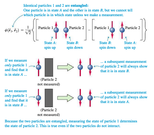
41.8 Quantum Entanglement
42 MOLECULES AND CONDENSED MATTER
42.1 Types Of Molecular Bonds
strong bonds (typical bond energies of 1 to 5 eV)
Ionic Bonds
ionization energy: \[ \mathrm{X}+\text { energy } \rightarrow \mathrm{X}^{+}+\mathrm{e}^{-} \]
electron affinity: \[ X+e^{-} \rightarrow X^{-}+\text { energy }\]
binding energy: energy needed to dissociate molecule into separate neutral atoms
Covalent Bonds
hybrid wave function
weaker bonds (typical energies are 0.1 eV or less)
van der Waals Bonds
from dipole–dipole interactions
Hydrogen Bonds
42.2 Molecular Spectra
Rotational energy levels
allowed transitions between rotational states must satisfy the same selection rule \(l\) must change by exactly one unit; that is, \(\Delta l = \pm 1\)
Vibrational energy levels
Rotation and vibration combined
| vibrational | rotational |
|---|---|
| each individual band in a spectrum | each individual line in a band |
| n-value | l-value |
molecules states = excited states of the electrons + rotational + vibrational states
When there is a transition between electronic states, the \(\Delta n = \pm 1\) selection rule for the vibrational levels no longer holds.
Complex Molecules

42.3 Structure of Solids
Crystal Lattices and Structures
Bonding in Solids
Types of Crystals
42.4 Energy Bands
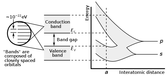
Insulators, Semiconductors, and Conductors

42.5 Free-Electron Model Of Metals
free-electron model
density of states
fermi–dirac distribution vs (Maxwell–Boltzmann distribution)
exclusion principle
indistinguishability
electron concentration and fermi energy
average free-electron energy
42.6 Semiconductors


42.7 Semiconductor Devices
1451